How Numba Enables Low-Level CUDA in Python: A Molecular Dynamics Showcase

August 14, 2026 56 minute read

In my previous post, I showed how JAX can be used to implement a GPU-accelerated MD simulator relying on just-in-time compilation, automatic vectorization, and automatic differentiation.

Have you ever wished you could write CUDA kernels without diving into C/C++? Numba-CUDA allows you write custom CUDA kernels directly in Python, giving you fine-grained control over GPU execution, from data movement to memory layouts, all while keeping the syntax simple. This is more than a basic wrapper around nvcc to compile kernels like CUDA C++. Numba compiles Python code, through LLVM and NVIDIA’s NVVM compiler infrastructure, to generate PTX code at runtime. Despite its excellent potential, Numba-CUDA remains in my opinion underappreciated. Many colleagues I’ve spoken with aren’t even aware it exists.

In this post, I’ll discuss fundamentals of CUDA kernels with Numba-CUDA and then put discussed concepts into practice by implementing a GPU-accelerated Molecular Dynamics simulator.

Let’s get started!

Writing and Executing CUDA kernel in Python with Numba-CUDA

To begin, I’ll cover basics of the CUDA execution model and memory hierarchy. If you’re already familiar with parallel programming on CPUs, many of the core concepts will feel familiar, making the transition to CUDA relatively straightforward.

How CUDA execution model enables parallelism

GPU speed up calculations through massive parallelism, where a large task is divided into smaller subtasks. These subtasks are distributed across hundreds or thousands of GPU cores and executed concurrently. In CUDA execution model, threads are the smallest execution units, performing individual computations. Additionally, blocks are groups of threads that can cooperate and synchronize. A grid is a collection of blocks, defining the full parallel scope of a kernel launch. The grid represent entire workload which enables scalable parallelism in CUDA, The underlying reasons for this hierarchical structure are related to hardware details. For example, threads within a block share fast on-chip memory and can communicate, but threads in different blocks cannot directly interact.

Diagram below shows an illustration of threads and blocks in a 1D grid:

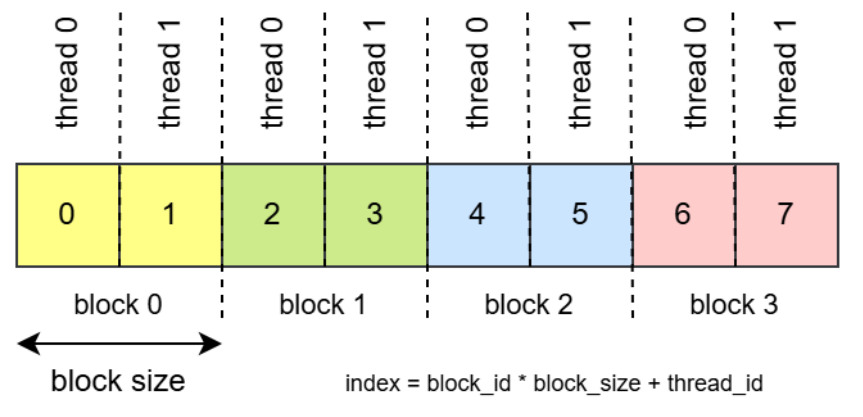
CUDA grid in 1D including threads and blocks

Each thread and block in kernel have their own assigned index to be identified. In this case, each block has 2 threads:

Block 0 → threads 0, 1 → indices 0, 1
Block 1 → threads 0, 1 → indices 2, 3
Block 2 → threads 0, 1 → indices 4, 5
Block 3 → threads 0, 1 → indices 6, 7

So each thread gets a unique global index which can be obtained using:

index = block_id × block_size + thread_id

This allows each CUDA thread to work on, for example, a different element of an array.

Writing a CUDA kernel

A kernel is the function that is executed by each thread in the CUDA grid. The kernel execution configuration defines how many threads are assigned to each block and how many blocks compose the gird. To create a CUDA kernel with numba.cuda, a Python function must be decorated with cuda.jit, as follows:

from numba import cuda

@cuda.jit
def my_cuda_kernel():
    ...

JIT (Just-In-Time) compilation means that code is compiled at runtime, when it is needed, rather than being fully compiled beforehand. Here, cuda.jit compiles the function into a CUDA GPU kernel when it is first called. Furthermore, Numba checks the argument types at runtime and dispatches the call to a matching compiled specialization; if non exists, JIT compilation creates one. This is called Dynamic dispatching which works together with JIT compilation.

Inside a running kernel, cuda.blockDim contains the shape of the blocks, cuda.blockIdx contains the position of the block with the running thread, and cuda.threadIdx contains the position of the running thread relative to its block. The global index in numba.cuda accordingly is written as

index = cuda.blockIdx.x * cuda.blockDim.x + cuda.threadIdx.x;

The .x means the x-dimension. CUDA supports 1D, 2D, and 3D grids and blocks.

Or, we can use numba-CUDA utility function

index = cuda.grid(1)

Where, 1 is for 1D grid. Respectively, ‘2’ and ‘3’ for 2D and 3D grids.

Let’s write a simple kernel that calculate an element-wise multiplication of two arrays:

from numba import cuda
from numpy.typing import NDArray 

@cuda.jit
def product_kernel(x: NDArray, y: NDArray, result: NDArray) -> None:
    idx = cuda.grid(1)
    if idx < len(x):
        result[idx] = x[idx] * y[idx]

Each GPU thread computes one element of the output array by calculating its global index with cuda.grid(1) and storing x[idx] * y[idx] in result[idx], while checking that the index is within the array bounds.

Numba-CUDA is currently in maintenance mode. New feature development is targeted towards Numba-CUDA-MLIR For migration guidance, see Migration from Numba / Numba-CUDA. In short, use from numba_cuda_mlir import cuda instead of from numba import cuda.

Executing the kernel

A CUDA kernel can be invoked and run on the GPU as follows:

kenrel[blocks_per_grid, threads_per_block](arguments)

The value between square bracket constitute the kernel launch configuration which determines the grid sizes. If the grid is 1D, these values are both integers. For 2D and 3D grid, these values must be tuples representing the number of threads and blocks per dimension.

We can easily run the product_kernel kernel, but first we need also preparing required input arrays

import numpy as np

x = np.linspace(0, 1, 1000, dtype=np.float32)
y = np.linspace(0, 1, 1000, dtype=np.float32)

The necessary data must be transferred from the host (the CPU and its memory) to the device (the GPU and its memory). The host is responsible for launching kernels, migrating data transfers, and allocating memory in device memory. After computation, the host can request to transfer the results back to host memory. Since CUDA kernel can only operate on arrays that reside in the memory of the GPU, this data must be copied to the device:

x_dev = cuda.to_device(x)
y_dev = cuda.to_device(y)
result_dev = cuda.device_array(x.shape, dtype=x.dtype)

Where, cuda.to_device method copies x (y) from CPU host memory to GPU device memory and cuda.device_array allocates an empty GPU array with the same shape and data type as x, intended to store the result. The x_dev, y_dev, and result_dev are device array whose data reside in the GPU’s memory. Device array can be passed to CUDA kernels, modified on the GPU, and later copy back to the host memory using .copy_to_host() method.

The final step is to determine the kernel launch configuration based on the problem size. We select a block size of 256 threads.

threads_per_block = 256

The grid must be of the same shape as the input and output arrays, since kernel mandates one-to-one mapping between thread and data elements. Therefore, the number of blocks in the grid is calculated as follows:

from math import ceil
blocks_per_grid = ceil(x.shape[0] / threads_per_block) 

The product_kernel can now be invoked as follows:

product_kernel[blocks_per_grid, threads_per_block](x_dev, y_dev, resutl_dev)

At the hardware level, GPU automatically distributing blocks across its multi-stream processors (SMs). Each block consists of many threads, which are further organized into groups of 32 threads called warps. A warp is the basic execution unit on the SM, meaning that its 32 threads execute the same instruction concurrently. An SM can have multiple blocks and warps active at the same time, depending on available resources such as registers and shared memory.

To see the result, the data must be copied back to the host:

result = result_dev.copy_to_host()

When a kernel is launched from the host (CPU), control is almost immediately returned to the host thread, even while the GPU is still executing the kernel. That means the host may continue executing before the GPU finishes its work This is called Asynchronous execution. If timing CUDA code, we must be careful that GPU operations are asynchronous by default. Adding cuda.synchronize() ensures that the timing includes the real GPU computation.

CUDA Memory Hierarchy

Another key concept is the CUDA memory hierarchy. GPUs expose several additional memory spaces to programmers, each with different storage capacity and performance characteristics. The most relevant ones for scientific computing are Global memory which is accessible by all threads. Shared memory is an on-chip memory region shared by all threads within the same block. Local memory is private to each thread. There are also specialized memory spaces such as Constant memory and Texture memory. These can be beneficial for specific access patterns but are generally less important for the types of scientific workloads considered in this post.

Diagram below shows CUDA memory hierarchy in a grid as follows:

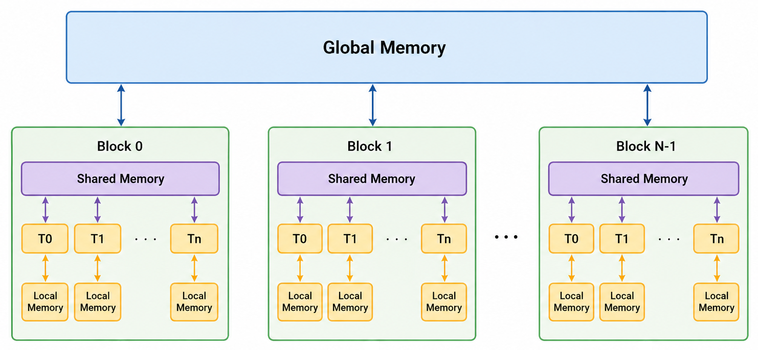
Each thread has its own set of registers as well, which are the fastest memory available on the GPU (latency of a few cycles). Although both registers and local memory are private to a single thread, they differ performance and physical location. Registers are stored directly on the GPU’s streaming multiprocessors (SMs) and provide the fastest possible access. Local memory, on the other hand, is conceptually private to a thread but is typically backed by device memory and therefore has much higher latency.

Each level of the memory hierarchy has its own constraints and usage patterns, which introduces additional complexity compared to CPU programming. So far, we have discussed the device memory which typically refers to global memory. This memory provides a large storage capacity, ranging from a few gigabytes to hundreds of gigabytes on modern accelerators, but it also has relatively high access latency compared to on-chip memory (1,000 versus 1-30 clock cycles). In the molecular dynamics application developed later in this post, we will store most simulation data in the global memory, while relying on local storage where appropriate for temporary force vector computations.

GPU Memory Access in Numbs-CUDA

Numba provides direct access to the GPU memory hierarchy, enabling explicit use of global, shared, and local memory spaces, each with different performance characteristics and use cases. Global memory is the large device memory accessible by all threads and is typically used to store the primary input and output data of a kernel:

array = cuda.device_array(1024, dtype=float32) 

Shared memory is a small but fast on-chip memory region that can be used for efficient data sharing among threads within the same thread block:

cache = cuda.shared.array(256, dtype=float32)

A common pattern is for each thread to load a value from global memory into shared memory, synchronize with the other threads in the block, and then reuse the cached data multiple times.

Local memory provides thread-private storage and is useful for temporary arrays required during a computation:

tmp = cuda.local.array(8, dtype=float32)

Although temporary scalar variables are usually placed in registers automatically by the compiler, local memory can be used when a thread requires its own private buffer.

Numba also supports atomic operations, which allow multiple threads to safely update the same memory location without introducing race conditions:

cuda.atomic.add(histogram, index, 1)

It increments the element histogram[index] by 1 while ensuring that concurrent updates from multiple threads are handled correctly. This is particularly useful for operations such as histograms, reductions, and counters.

Numba also allows interoperability between Numba device array and other GPU-enabled libraries such as CuPy enabling data to be exchanged without copying it back to the CPU (zero-copy). This makes it possible to combine custom CUDA kernels written in Python with high-level GPU libraries in a single application. Example of zero-copy conversion from a Numba device array to a CuPy array: x_cupy = cupy.asarray(x_numba).

Now, let’s put what have discussed into practice by creating a GPU-accelerated molecular dynamics (MD) simulator which is used for studying materials at the atomic scale. We’ll begin with a high-level overview of how MD simulation works, then we will implement the necessary components step by step while using the features provided by Numba-CUDA.

Implementing a GPU-Accelerated Molecular Dynamics Simulator

Molecular Dynamics (MD) is a technique often used for predicting the behavior of materials at the atomic scale. We will simulate a simple atomic system of an ideal gas, such as helium, in two dimensions, to minimize complex technical details that may require specialized expertise. As our main focus, Numba CUDA will be used to accelerate the computationally demanding kernels, including the particle-particle interactions and time integration. MD simulation can be broken down into four main steps:

System initialization initializes the state of our collection of particles and choosing simulation settings.
Atomic interactions calculates the interactions between the particles, which determine how particles move in response to forces.
Time integration determines how the particles move over time via solving Newton’s equations of motion for each particle.
Data collection: saves a subset of the information which must be periodically extracted for on-the-fly or later analysis.

In the system initialization step, we will allocate and initialize the necessary arrays on the GPU memory. In the atomic interactions and time integration steps, we will implement CUDA kernels to compute the forces and update the particles, respectively. Finally, the last step transfers data to the host for further analysis. The flowchart below illustrates how the various components of MD simulations fit together.

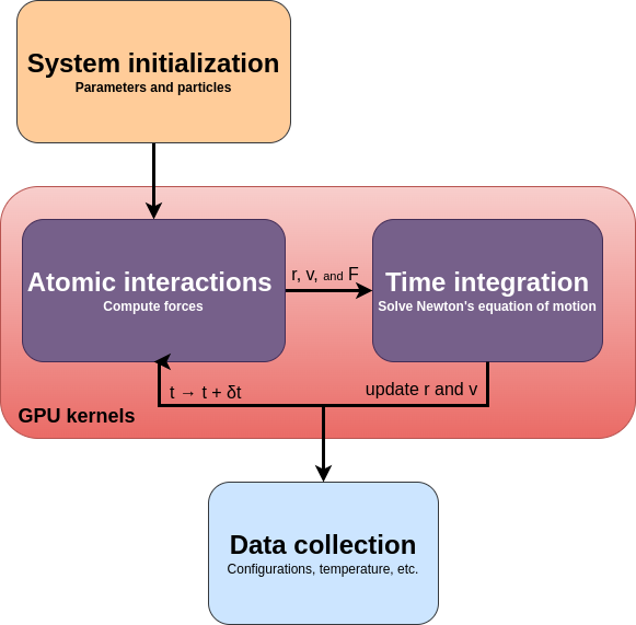
Key components in molecular dynamics (MD) simulation.

Time is discretized into small intervals called time step ($\delta t$). For each time step, there is an iterative process between force calculations and the time integration, which updates the positions and velocities of the particles. This process is repeated iteratively to obtain the trajectories of the particles over time.

In what follows, I will elaborate on each step and create an implementation for each.

1. System initialization

The system we want to model is a collection of particles (or atoms). Particles are initialized with starting positions and velocities, based on experimental data and physical conditions such as desired temperature and pressure. In an MD simulation, particles are constrained to a finite region of space called a simulation box. To mimic an infinite system, which is a good approximation for real liquids, gases, and bulk materials, the boundaries of this box are usually defined to be periodic. This means that when an atom moves outside one boundary, it reappears on the opposite side, mimicking continuous space. Here, we consider a system composed of a single type of atom positioned within a 2D box. This setup restricts the particles to movement in the x-y plane; motion along the z-axis is not allowed.

Simulation parameters

First of all, we need to import numpy and numba.cuda.We also import some types and define some aliases for type annotations, which helps to improve code readability.

import math
import numpy as np
from numba import cuda
from numpy.typing import NDArray
from typing import TypeAlias, TextIO

FLOAT: TypeAlias = np.float64
Array: TypeAlias = NDArray[FLOAT]

In scientific simulations, float64 precision is usually prefered to reduce numerical instability due to the accumulation of round-off errors. However, there are reasons to prefer float32 precision. GPUs are usually hardware optimized for 32-bit operations, so using float32 generally results in better performance. float32 requires half the number of bytes compared to float64, so it is more economical with respect to memory usage and bandwidth. To be flexible, we defined an alias FLOAT which we can set to either float32 or float64. Additionally, we define the alias Array for multidimensional arrays that can hold elements of the type specified by FLOAT.

Next, we define system parameters using a named tuple, which allowing us to create an immutable data structure with named fields. This is quite similar to a C-like struct and very useful for passing related data into Python functions with a single argument. More importantly, numba.cuda JIT-compiled functions accept tuple and named tuples as input argument.

from typing import NamedTuple, TypeAlias, TextIO

class SimulationParameters(NamedTuple):
    num_atoms: int
    time_step: float
    box_length: float
    atom_spacing: float
    velocity_std: float 

In our simulation, we will set the number of atoms num_atoms=100 and the initial atom spacing atom_spacing=2.5. The time_step represents the interval between simulation updates and is set to 0.0001. The simulation box side length box_length is calculated based on the number of atoms and their spacing. Finally, the velocity standard deviation velocity_std is set to 10.0.

num_atoms = 100
atom_spacing = 2.5     

params = SimulationParameters(
    num_atoms=num_atoms,
    time_step=0.0001,
    box_length=math.sqrt(num_atoms) * atom_spacing,
    atom_spacing=atom_spacing,
    velocity_std=10.0,
)

To set the box length, we considered both the number of atoms and the spacing between nearest neighbors. In general, atoms can be distributed evenly within a box using the formula $N^{1/dim} \times \text{atom spacing}$, where N is the number of atoms and dim represents the dimension of the box. In our case, since the dimension is 2, we use the square root.

In our demo system these values don’t have a real meaning since we don’t use any units. In real-world simulations, these parameters have units and their value needs to be determined based on experiments or other types of calculations.

Particles

We define an additional named tuple Particles, which will store positions, velocities, and forces of all particles in form of arrays with the shape (num_atoms, dim). Since we simulate a 2D system dim=2. Our example can be easily extended to a 3D system.

class Particles(NamedTuple):
    position: Array
    velocity: Array
    force: Array

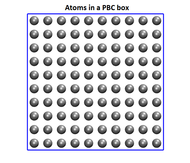
We implement two functions to set up the initial conditions: one for the positions and one for the velocities. The initialize_position function distributes the atoms on a square lattice in the 2D box, so that each atom is equidistant to its nearest neighbors.

def initialize_position(
    params: SimulationParameters,
) -> Array:
    atom_spacing = params.atom_spacing
    num_atoms_per_row = math.ceil(math.sqrt(params.num_atoms))
    position = np.empty(shape=(params.num_atoms, 2), dtype=FLOAT)
    atom_index = 0
    for index_j in range(num_atoms_per_row):
        for index_i in range(num_atoms_per_row):
            if atom_index < position.shape[0]:
                position[atom_index, 0] = (index_i + 0.5) * atom_spacing
                position[atom_index, 1] = (index_j + 0.5) * atom_spacing
            atom_index += 1
    return position

We displace all the atoms by half of the lattice spacing to center them in the simulation box. Due to periodic boundary conditions, this is somewhat arbitrary, but we don’t want our atoms to start on the boundary. Note that the initial positioning does not reflect a realistic physical arrangement, it is simply a way used to distribute atoms without causing overlaps.

The initial configuration of 100 atoms in a periodic simulation box.

Second, initialize_velocity assigns random initial velocities to all atoms. The velocities are sampled from a 2D standard normal distribution which is scaled by the velocity_std parameter. Randomizing the velocities ensures that the atoms start with a range of initial kinetic energies, like a thermal motion in the system. The velocities are adjusted by subtracting the mean velocity in each $x$ and $y$ directions (axis=0), centering the velocity distribution around zero, to ensure that the system’s center of mass remains constant.

def initialize_velocity(
    params: SimulationParameters,
    rng: np.random.Generator,
) -> Array:
    velocity = rng.normal(size=(params.num_atoms, 2)).astype(FLOAT)
    velocity *= params.velocity_std
    velocity -= velocity.mean(axis=0)
    return velocity

The velocities are adjusted by subtracting the mean velocity in each $x$ and $y$ directions (axis=0), centering the velocity distribution around zero, to ensure that the system’s center of mass remains constant.

With these two initialization functions in place, we can now proceed to create Particles on the device as shown below:

position = initialize_position(params)
position_dev = cuda.device_array(position.shape, dtype=FLOAT, order="F")
cuda.to_device(position, to=position_dev)

rng = np.random.default_rng(1234)
velocity = initialize_velocity(params, rng)
velocity_dev = cuda.device_array(velocity.shape, dtype=FLOAT, order="F")
cuda.to_device(velocity, to=velocity_dev)

force_dev = cuda.device_array(shape=(num_atoms, 2), dtype=FLOAT, order="F")
particles = Particles(position_dev, velocity_dev, force_dev)

We initialize the position and velocity on the host and copy them to the device. The force array does not need initial values, as it will be computed later based on the atom positions. This array is simply allocated on the device. For the device arrays we select column major (F) memory layout rather than the default row major (C). For the CUDA kernels we will define, this alignment minimizes global memory accesses because threads in the same warp access contiguous memory addresses. This coalesced data arrangement will improve the performance on the GPU.

2. Atomic interactions

Potential energy determines how particles interact in any physical system. Like water that flows downhill, a system tends to evolve to a state of minimal potential. Forces experienced by particles can be derived from the negative gradient of the potential respect to their positions. Forces give rise to motion of the particles, and this will be a direction that reduces the potential. To calculate the potential energy between atoms, we use a set of mathematical functions and parameters. It captures the effects of bonded and non-bonded interaction between atoms as a function of their separation distance. The parameters for a potential are obtained from either experimental data or quantum mechanical calculations.

Lennard-Jones forces

The force vector in a Lennard-Jones system $\vec{F}_{ij}$ on particle $i$ due to particle $j$ is given by:

\[\vec{F}_{ij}^{} = 24 \epsilon \left[ 2(\frac{\sigma}{r_{ij}})^{12} - (\frac{\sigma}{r_{ij}})^{6} \right] \frac{\vec{r}_{ij}}{r_{ij}^{2}}\]

Where, $\vec{r}_{ij} = \vec{r}_i - \vec{r}_j$ represents the vector pointing from particle $j$ to particle $i$.

For the total force on particle $i$, we sum the contributions from all other particles $j$:

\[\vec{F}_i = \sum_{j=1, i\neq j}^{N} \vec{F}_{ij}\]

This will give us the net force acting on particle $i$ due to all other particles in the system while excluding the self interaction.

Parallelizing the force calculations

We will write a CUDA kernel to calculate forces for each particle in parallel by mapping each calculation onto a separate thread. This is feasible because force calculations for individual atoms are independent and can be easily executed as embarrassingly parallel tasks. Each thread reads all the positions from global memory and updates its own forces without causing race conditions, as each element in the force array is written to by only one thread. This allows us to eliminate the need for a loop over the atom index, enabling threads in the grid to run these calculations concurrently.

The following implementation shows how to distribute force calculation tasks across multiple GPU threads:

@cuda.jit
def compute_force(
    particles: Particles,
    params: SimulationParameters,
) -> None:
    force = cuda.local.array(shape=(2,), dtype=FLOAT)
    start, stride = cuda.grid(1), cuda.gridsize(1)
    for index_i in range(start, params.num_atoms, stride):
        ri = particles.position[index_i]
        fi = particles.force[index_i]
        # calculate per atom force
        force[0], force[1] = 0.0, 0.0
        for index_j in range(params.num_atoms):
            if index_i != index_j:
                rj = particles.position[index_j]
                pair_interaction(ri, rj, params.box_length, force)
        fi[0], fi[1] = force[0], force[1]

We first allocated an array force with shape=(2,) in the GPU local memory (using register instead?). Each thread computes the net force acting on one or multiple atoms based on index_i. The loop over index_i ensures that each thread receives the correct index within the grid, even if the number of atoms exceeds the grid size. This can occur in very large systems containing many atoms. When params.num_atoms>stride, one thread will handle multiple atoms sequentially.

The inner loop over index_j iterates over all other atoms, excluding the atom itself (index_i != index_j). For each pair of atoms, the pair_interaction device function is called to compute the force between atom $i$ (ri) and atom $j$ (rj), and the results are added to the local force array. After summing the forces from all other atoms $j$, the results from the local force array are written to the particles.force array in global memory.

The pair_interaction function calculates the force exerted between two atoms $i$ and $j$ based on their positions. It implements the force derived from the Lennard-Jones potential. We decorate this function with @cuda.jit(device=True), meaning it can be called as a device function within the compute_force CUDA kernel. Splitting out device functions helps us make kernels more modular and readable.

@cuda.jit(device=True)
def pair_interaction(
    position_i: Array,
    position_j: Array,
    box_length: FLOAT,
    force: Array,
) -> None:
    rij_x = apply_pbc(position_i[0] - position_j[0], box_length)
    rij_y = apply_pbc(position_i[1] - position_j[1], box_length)
    r2 = rij_x * rij_x + rij_y * rij_y
    r2i = 1.0 / r2         
    r6i = r2i * r2i * r2i  
    coef = 24.0 * r6i * (2.0 * r6i - 1.0) 
    force[0] += rij_x * r2i * coef
    force[1] += rij_y * r2i * coef

Here, we use apply_pbc function for each dimension, to enforce periodic boundary conditions. This corrects the distance calculation so that atoms on opposite edges of the simulation box still interact correctly.

For optimization reasons, we use r2 instead or r to avoid calling the computationally expensive square root function. Similarly, since division is generally more time-consuming than multiplication, we also use a temporary variable r2i to store the inverse of r2.

@cuda.jit(device=True, inline=True)
def apply_pbc(
    rij: FLOAT, 
    box_length: FLOAT,
) -> FLOAT:
    L = box_length
    if rij >= 0.5 * L:
        rij -= L
    elif rij <= -0.5 * L:
        rij += L
    return rij

For the apply_pbc device function, we pass the inline=True argument to specify that it should be also inlined. When a function is inlined, the compiler inserts the function’s code directly into the calling code, rather than making a separate function call. This can improve performance by reducing function call overhead, and is always recommended for very small functions.

The conditional block adjusts the value of $r_{ij}$ by applying periodic boundary conditions, wrapping it around to the negative or positive side when necessary. Finally, the function returns the modified value of $r_{ij}$.

At this point, we have a ready-to-use kernel that calculates forces for all the atoms in the simulation box in parallel. In the next section, we will learn how to update atomic positions and velocities for a next time step.

3. Time integration

Time integrator updates the positions and velocities of atoms as time in the simulation progresses. In principle it numerically solves Newton’s equations of motion for each atom in the system.

Verlet integrator

The Verlet algorithm is one of the simplest and most commonly used time integrators in MD simulations because of its simplicity, computational efficiency, and numerical stability. In Verlet integration the new position $\vec{r}(t+\delta t)$ of a particle is computed based on its current and previous positions as follows:

\[\vec{r}(t+\delta t) = \vec{r}(t) + \vec{v}(t) \delta t + \frac{1}{2} \vec{a}(t) \delta t^2\]

Where, $\vec{r}(t)$, $\vec{v}(t)$, and $a(t)$ are the position, velocity and the acceleration of the atom at the current time, and $\delta t$ is the time step. Acceleration $\vec{a}$ relates to Newton’s law via $\vec{F}=m\vec{a}$, where $\vec{F}$ is the force and $m$ is the mass. For our particles, we will take $m=1$, which makes $\vec{F}=\vec{a}$.

The equation for the updated velocity $\vec{v}(t+\delta t)$ is given by:

\[\vec{v}(t+\delta t) = \vec{v}(t) + \frac{1}{2} \left[ \vec{a}(t) + \vec{a}(t + \delta t) \right] \delta t\]

The positions and velocities for all atoms are updated, and the algorithm proceeds to the next time step $t \rightarrow t + \delta t$. This process repeats, with forces recalculated at each step to gradually build the trajectory of the particles.

Parallelizing the integrator

We’ll follow the same approach to speed up the time integration as we used to calculate the forces: we parallelize over the all the atoms. CUDA kernel below updates the position of atoms:

@cuda.jit
def verlet_integration_position(
    particles: Particles, 
    params: SimulationParameters,
) -> None:
    r, v, f = particles
    dt, L = params.time_step, params.box_length
    start, stride = cuda.grid(1), cuda.gridsize(1)
    for index in range(start, params.num_atoms, stride):
        for dim in range(2):
            r[index, dim] = math.fmod(
                r[index, dim] + dt * (v[index, dim] + 0.5 * dt * f[index, dim]) + 10.0 * L,
                L,
            )
            v[index, dim] += 0.5 * dt * f[index, dim]

The new position r[idx, dim] is obtained using the current velocity and force values according to Equation 5. The x and y position can be updated independently, so we have an inner loop for the dimensions. The additional term 10.0 * L ensures that the position remains within the bounds of the simulation box [0, L) after updating. This is followed by math.fmod(..., L) to enforce periodic boundary conditions, ensuring that atoms wrap around if they go outside the simulation box. This step is crucial because without it, new positions could potentially become negative, which can lead to issues when applying periodic boundary conditions.

Notice that the velocity v[idx, dim] is already partially updated at this step. It will be updated second time, once the new forces are calculated in the next integration step (see Equation 6). We iterate over all the atom indices using the start and stride, allowing each thread to update multiple atoms if the grid size is smaller than the number of atoms.

We do the same thing for the final update to the velocity. The following kernel is invoked once the forces are updated with the new positions:

@cuda.jit
def verlet_integration_velocity(
    particles: Particles, 
    params: SimulationParameters,
) -> None:
    v, f = particles.velocity, particles.force
    dt = params.time_step
    start, stride = cuda.grid(1), cuda.gridsize(1)
    for index in range(start, params.num_atoms, stride):
        for dim in range(2):
            v[index, dim] += 0.5 * dt * f[index, dim]

4. Data collection

A large amount of data is generated from an MD system including atomic positions, velocities, and forces. This information can be used to track atomic motions, identify interactions, and calculate physical properties like energies, temperature, and pressure. However, so far we don’t have any way to save the output of our simulation. To allow us to post-process and visualize our data, we define a save function which dumps the atomic position data into a file in the XYZ format. This is a standard way to represent molecular structures, making it compatible with various visualization tools such as the VMD package.

def save(position: Array, file: TextIO) -> None:
    num_atoms = position.shape[0]
    file.write(f"{num_atoms}\n\n")
    for i in range(num_atoms):
        file.write(f"{'He'}\t{position[i, 0]} {position[i, 1]} {0}\n")
    file.flush()

The line with file.flush() ensures that all data is immediately written to the file. Additionally, we calculate temperature ($T$) which is directly related to the average kinetic energy of the atoms within the system.

\[T \propto \frac{1}{N} \sum_{i=1}^{N} \frac{1}{2} m \vec{v}_i^{2}\]

This equation calculates the average kinetic energy of atoms in a system. $\vec{v}_i$ represents the velocity of atom number i, and m is the mass which we have assumed to be equal to $1.0$. Calculating the temperature of the system is done with the get_temperature function as follows:

def get_temperature(velocity: Array) -> FLOAT:
    return 0.5 * (velocity**2).sum() / velocity.shape[0]

Running the MD simulation

Finally, we connect all the different pieces in the simulate function to run our MD simulation. We will iteratively apply these force and time integration kernels within a for loop, enabling us to run the MD simulation.

def simulate(
    params: SimulationParameters,
    particles: Particles,
    steps: int = 1,
    log_frequency: int = 100,
    filename: str = "configurations.xyz",
) -> None:
    print("GPU-accelerated Molecular Dynamics Simulation")
    print("Lennard-Jones Particles in a 2D Periodic Box")
    print(f"Number of atoms: {params.num_atoms}")
    print("Step    Time         Temperature")
    print("--------------------------------")
    threads = 32
    blocks = math.ceil(params.num_atoms / threads)
    compute_force[blocks, threads](particles, params)
    with open(filename, "w") as file:
        # Simulate
        for step in range(steps):
            if step % log_frequency == 0:
                temperature= get_temperature(particles.velocity.copy_to_host())
                print(
                    f"{step:<7d}"
                    f" {step * params.time_step:<12.8f}"
                    f" { temperature:<.8f}"
                )
                save(particles.position.copy_to_host(), file)
            # Next time step (update r, v, and F)
            verlet_integration_position[blocks, threads](particles, params)
            compute_force[blocks, threads](particles, params)
            verlet_integration_velocity[blocks, threads](particles, params)
    print("Done.")

This function simulates the system for predefined number of time steps, allowing the particle positions to evolve in accordance with the Lennard Jones potential. Over time, the system tends to reach an equilibrium state where properties (i.e., temperature) stabilize. We also collect properties like position of atoms and temperature during the simulation. We simulate the system for the next 1000 time steps and collecting current temperature and save atom positions every $100$ steps.

simulate(params, particles, steps=1000)

Output:

GPU-accelerated Molecular Dynamics Simulation
Lennard-Jones Particles in a 2D Periodic Box
Number of atoms: 100
Step Time Temperature
--------------------------------
0 0.00000000 95.76379342
100 0.01000000 95.76576249
200 0.02000000 95.77276531
...
900 0.09000000 95.79469347
Done.

A complete working example of the GPU-accelerated MD simulator is provided in this jupyer notebook.

Benchmarks

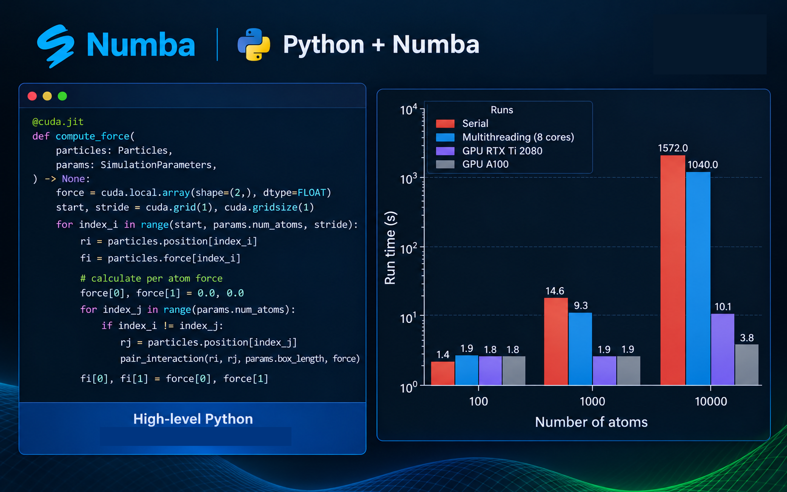
To illustrate the runtime performance of our GPU implementation of an MD simulator, I ran it for different system sizes of 100, 1,000, and 10,000 atoms and compare to two CPU implementations:

A serial version of the same code optimized with Numba’s just-in-time compilation.
A parallel version on an 8-core CPU using Numba’s JIT along with prange for multi-threading.

The GPU version was run on A100, a data center GPU, and additionally RTX Ti 2080, a consumer GPU. The following figure shows the elapsed runtime. Note that the y axis is logarithmically scaled, and precision is in float64.

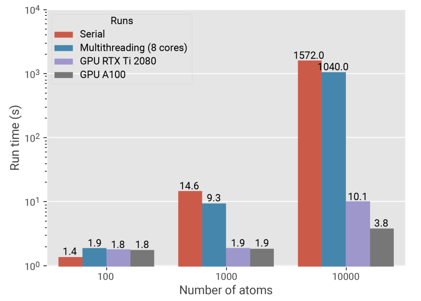
Our MD simulation benchmark runs on a different system for 1,000 time steps

For small systems, GPU computing offers few benefits due to its overhead and GPU underutilization. For large systems, the performance gains with the GPU are significant. The RTX GPU achieved up to 150x faster than the serial code, and the A100 GPU was nearly 400x faster. The significant difference in performance between the two GPU types is due to the higher computing capacity and the hardware support for floating-point operations in the data center GPU.

At the algorithmic level, we have used a basic approach to identify neighboring atoms by looping over all atoms, resulting in a computational complexity of $O(N^2)$, where $N$ is the number of atoms. Advanced methods like neighbor lists together with linked-cell algorithms can reduce this complexity to $O(N)$, enabling MD simulations to efficiently handle larger systems with millions of atoms. I’ll discuss the linear scaling MD in a separate post in near future.